SGMs：基于分数的生成模型

扩散模型是一类概率生成模型，它通过注入噪声逐步破坏数据，然后学习其逆过程，以生成样本。目前，扩散模型主要有三种形式：去噪扩散概率模型[2,3] (Denoising Diffusion Probabilistic Models, 简称DDPMs)、基于分数的生成模型[4,5] (Score-Based Generative Models,简称SGMs)、随机微分方程[6,7,8] (Stochastic Differential Equations,简称Score SDEs)。

SGMs

根据文献[4]，可知，与基于似然方式的生成模型和生成式对抗模型不同，基于分数的生成模型不需要对抗训练，也不需要在训练时采样。首先，它需要近似高斯噪声扰动后数据梯度的分布函数；然后，利用Annealed Langevin Dynamics生成样本。接下来，利用数学语言描述基于分数的生成模型。

假设从未知数据分布$p_{data}(\mathbf{x})$采样得到独立同分布的数据集$\{\mathbf{x}_i\in\mathbb{R}^D\}_{i=1}^N$。同时，定义

概率密度$p(\mathbf{x})$的分数为$\nabla_{\mathbf{x}}log{p(\mathbf{x})}$
分数网络$\mathbf{s}_{\theta}:\mathbb{R}^D\to\mathbb{R}^D$是一个参数化的神经网络，用于近似$p_{data}(\mathbf{x})$分数

生成模型的目标是学习一个生成服从分布$p_{data}(\mathbf{x})$的新样本，那么目标函数为
$$
\begin{aligned}
\frac{1}{2}\mathbb{E}_{p_{data}}[\Vert\mathbf{s}_{\theta}(\mathbf{x}）-\nabla_{\mathbf{x}}log{p_{data}}(\mathbf{x})\Vert_2^2]=\mathbb{E}_{p_{data}(\mathbf{x})}[tr(\nabla_{\mathbf{x}}\mathbf{s}_{\mathbf{\theta}}(\mathbf{x})) \\
+\frac{1}{2}\Vert\mathbf{s}_{\theta}(\mathbf{x})\Vert_2^2]+CONSTANT
\end{aligned}\tag{1}
$$
式(1)中$\nabla_{\mathbf{x}}\mathbf{s}_{\theta}(\mathbf{x})$为$\mathbf{s}_{\mathbf{\theta}}(\mathbf{x})$的雅可比矩阵。然而，求解该目标函数会遇到以下挑战：

由于雅可比矩阵迹计算复杂，分数匹配无法扩展到深度神经网络和高维数据。
由于现实任务的数据往往处于低维流形，数据分布的梯度是未定义的。
在数据分布密度低的区域，往往因数据不足造成估计不准确。
若数据分布的两种模式被低密度区域分开，Langevin Dynamics无法在有限时间内恢复两种模式的相对权重。

由于高斯分布梯度计算很方便，所以解决了雅可比矩阵计算复杂的问题。同时，数据扰动也能解决数据分布处于低维流形的问题，也减少了数据分布密度低的问题。为了解决Langevin Dynamics无法区分数据模式权重的问题，利用annealed Langevin Dynamics进行数据生成。

若$\sigma_i$为高斯分布的方差，且集合$\{\sigma_i\}_{i=1}^L$中元素满足$\frac{\sigma_1}{\sigma_2}=\cdots=\frac{\sigma_{L-1}}{\sigma_L}\gt1$，那么扰动后的数据分布为$q_{\sigma}(\mathbf{x})=\int p_{data}(\mathbf{t})\mathcal{N}(\mathbf{x}\vert\mathbf{t},\sigma^2I)d\mathbf{t}$。同时，为了应对以上挑战，$\sigma_1$应足够的大以缓和梯度计算的困难，$\sigma_L$应足够小以减少对数据的影响。分数网络应该用于估计数据扰动后分布的梯度，即$\forall\sigma\in\{\sigma_i\}_{i=1}^L:\mathbf{s}_{\theta}(\mathbf{x},\sigma)\approx\nabla_{\mathbf{x}}log{q_{\sigma}(\mathbf{x})}$。此时，$\mathbf{s}_{\theta}(\mathbf{x},\sigma)$称为Noise Conditional Score Network(NCSN)，对于每个给定的$\sigma$，目标函数为
$$
\begin{aligned}
l(\theta;\sigma)=\frac{1}{2}\mathbb{E}_{p_{data}(\mathbf{x})}\mathbb{E}_{\tilde{x}\sim\mathcal{N}(\mathbf{x},\sigma^2 I)}[\Vert\mathbf{s}_{\theta}(\tilde{\mathbf{x}},\sigma)+\frac{\tilde{\mathbf{x}}-\mathbf{x}}{\sigma^2}\Vert_2^2]
\end{aligned}\tag{2}
$$
对于所有的$\sigma_i$，损失函数为
$$
\begin{aligned}
\mathcal{L}(\mathbf{\theta};\{\sigma_i\}_{i=1}^L)=\frac{1}{L}\sum_{i=1}^{L}\lambda(\sigma_i)l(\mathbf{\theta};\sigma_i)
\end{aligned}\tag{3}
$$
式(3)中$\lambda(\sigma_i)=\sigma_i^2$，以便于每项$\lambda(\sigma_i)l(\mathbf{\theta};\sigma_i)$为同一个数量级。以此为目标函数训练神经网络，就可以得到数据分布梯度的估计函数。

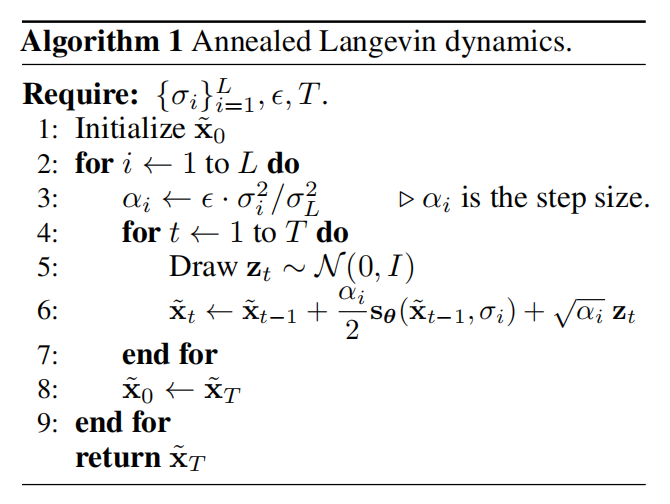
基于分数估计函数，可利用Annealed Langevin dynamics算法生成样本，可见算法1所示。

文献[4]提出的基于分数的生成模型虽然能够生成高质量的样本。然而，根据文献[5]，可知，该方法不能扩展到高维特征，且在某些场景下不稳定。因此，需要对基于分数的生成模型改进，可改进的方面有

高斯噪音的方差$\{\sigma_{i}\}_{i=1}^L$的设定
分数网络$\mathbf{s}_{\theta}(\mathbf{x},\sigma)$包含参数$\sigma$的方式
步长参数$\epsilon$的设定
采样步数$T$

算法优化

正态噪音方差的选择

对于初始噪音方差$\sigma_1$的选择，文献[4]提出应与训练数据中数据对之间欧氏距离一样大；噪音方差$\sigma_{L}$为0.01，保持不变；对于其它的噪音方差的选择，应符合以$\gamma=\frac{\sigma_{i-1}}{\sigma}$为比例的等比数列，且满足式(16)
$$
\begin{aligned}
\Phi(\sqrt{2D}(\gamma-1)+3\gamma)-\Phi(\sqrt{2D}(\gamma-1)-3\gamma)\approx0.5
\end{aligned}\tag{4}
$$
式(4)中$\Phi$为标准正态分布，$D$为数据维度。

分数网络包含噪音信息的方式

文献[4]中分数网络是以方差$\sigma$为条件的网络，那么对于无归一化的分数网络，其内存的需求与$L$呈现线性关系，这是不适用的。因此，$\mathbf{s}_{\theta}(\mathbf{x},\sigma)=\mathbf{s}_{\theta}(\mathbf{x})/\sigma$是一种简单高效的替代方式，$\mathbf{s}_{\theta}(\mathbf{x})$为无条件分数网络。

退火朗之万动力学参数配置

命题1：若令$\gamma=\frac{\sigma_{i-1}}{\sigma_{i}}$,$\alpha=\epsilon\cdot\frac{\sigma_i^2}{\sigma_L^2}$，利用算法1，生成数据满足$\mathbf{x}_{T}\sim\mathcal{N}(0,s_t^2\mathbf{I})$。其中
$$
\begin{aligned}
\frac{s_T^2}{\sigma_i^2}=(1-\frac{\epsilon}{\sigma^2_L})^{2T}(\gamma^2-\frac{2\epsilon}{\sigma_L^2-\sigma_L^2(1-\frac{\epsilon}{\sigma_L^2})^2})+\frac{2\epsilon}{\sigma_L^2-\sigma_L^2(1-\frac{\epsilon}{\sigma_L^2})^2}
\end{aligned}\tag{5}
$$
根据式(5)，可知，$\forall i\in(1,T]$，$\frac{s^2_T}{\sigma_i^2}$相等。

若期望$\frac{s^2_T}{\sigma_i^2}\approx1$，那么可先根据计算资源选择尽可能大的$T$，然后选择$\epsilon$使其尽可能$\frac{s^2_T}{\sigma_i^2}$尽可能接近1。

移动平均提升稳定性

虽然基于分数的生成模型，不需要对抗训练，但是仍会出现训练不稳定、颜色偏移的问题。然而，这个问题可通过指数移动平均解决。指数移动平均是指在训练分数网络时，参数更新方式为
$$
\begin{aligned}
{\mathbf{\theta}}'\leftarrow m{\mathbf{\theta}}'+(1-m){\mathbf{\theta}_i}
\end{aligned}\tag{6}
$$
式(6)中$\theta_i$为第$i$次模型训练之后的模型参数，${\theta}'$为第$i-1$次训练之后的模型参数，$m$为动量参数。

参考文献

[1] Yang L, Zhang Z, Song Y, et al. Diffusion models: A comprehensive survey of methods and applications[J]. ACM Computing Surveys, 2023, 56(4): 1-39.

[2] Ho J, Jain A, Abbeel P. Denoising diffusion probabilistic models[J]. Advances in neural information processing systems, 2020, 33: 6840-6851.

[3] Sohl-Dickstein J, Weiss E, Maheswaranathan N, et al. Deep unsupervised learning using nonequilibrium thermodynamics[C]//International conference on machine learning. PMLR, 2015: 2256-2265.

[4] Song Y, Ermon S. Generative modeling by estimating gradients of the data distribution[J]. Advances in neural information processing systems, 2019, 32.

[5] Song Y, Ermon S. Improved techniques for training score-based generative models[J]. Advances in neural information processing systems, 2020, 33: 12438-12448.

[6] Song Y, Sohl-Dickstein J, Kingma D P, et al. Score-based generative modeling through stochastic differential equations[J]. arXiv preprint arXiv:2011.13456, 2020.

[7] Song Y, Durkan C, Murray I, et al. Maximum likelihood training of score-based diffusion models[J]. Advances in Neural Information Processing Systems, 2021, 34: 1415-1428.

[8] Karras T, Aittala M, Aila T, et al. Elucidating the design space of diffusion-based generative models[J]. Advances in Neural Information Processing Systems, 2022, 35: 26565-26577.

[9] Rao–Blackwell theorem - Wikipedia

[10] Evidence lower bound - Wikipedia

[11] Generative Modeling by Estimating Gradients of the Data Distribution | Yang Song (yang-song.net)

[12] Itô diffusion - Wikipedia