DDPM：去噪扩散概率模型

扩散模型是一类概率生成模型，它通过注入噪声逐步破坏数据，然后学习其逆过程，以生成样本。目前，扩散模型主要有三种形式：去噪扩散概率模型$[2,3]$ (Denoising Diffusion Probabilistic Models, 简称DDPMs)、基于分数的生成模型$[4,5]$ (Score-Based Generative Models,简称SGMs)、随机微分方程$[6,7,8]$(Stochastic Differential Equations,简称Score SDEs)。

DDPMs

扩散概率模型是一个被参数化的马尔科夫链，在有限时间内通过变分推断训练模型生成样本。它的学习范式可分为两个过程，一个是不断的向样本数据中加入高斯噪音直至破坏样本的扩散过程；另一个是逆扩散过程，也称逆过程，该过程需要学习马尔科夫链中状态之间的转换函数。如图1所示，扩散模型的有向图模型。

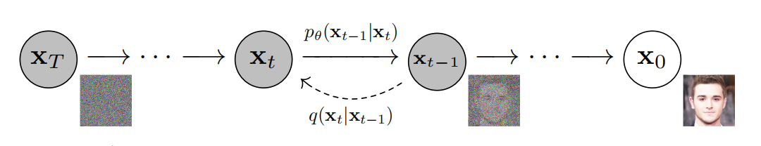
根据图1，可知，扩散图模型是隐变量模型，其数学表达可见式(1)。其中，$\mathbf{x}_1,\dots,\mathbf{x}_T$是与$\mathbf{x}_0\sim q(\mathbf{x}_0)$维度相同的隐变量。

$$ \begin{equation} p_{\theta}(\mathbf{x}_0):=\int p_{\theta}(\mathbf{x}_{0:T})d\mathbf{x}_{1:T} \tag{1} \end{equation} $$

其中，联合分布$p_{\theta}(\mathbf{x}_{0:T})$为逆过程。逆过程中马尔科夫链之间的转换函数$p_{\theta}(\mathbf{x}_t)$为高斯分布。若起始点$T$的分布函数为$p(\mathbf{x}_T)=\mathcal{N}(\mathbf{x}_T;0,\mathbf{I})$，那么

$$ \begin{equation} p_{\theta}(\mathbf{x}_{0:T}):=p(\mathbf{x}_T)\prod_{t=1}^Tp_{\theta}(\mathbf{x}_{t-1}\vert\mathbf{x}_t),\qquad p_{\theta}(\mathbf{x}_{t-1}\vert\mathbf{x}_t):=\mathcal{N}(\mathbf{x}_{t-1};\mu_{\theta}(\mathbf{x}_{t-1},t),\Sigma_{\theta}(\mathbf{x}_t,t))\tag{2} \end{equation} $$

与其它隐变量不同，扩散模型的近似后验$q(\mathbf{x}_{1:T}\vert\mathbf{x}_0)$，被称为前向过程或扩散过程，是一个固定的马尔科夫链。扩散过程是一个向数据中按照方差为$\beta_1,\dots,\beta_{T}$顺序不断增加高斯噪音的过程。

$$ \begin{equation} q(\mathbf{x}_{1:T}\vert\mathbf{x}_0):=\prod_{t=1}^T q(\mathbf{x}_t\vert\mathbf{x}_{t-1}),\qquad q(\mathbf{x}_t\vert\mathbf{x}_{t-1}):=\mathcal{N}(\mathbf{x}_t;\sqrt{1-\beta_t}\mathbf{x}_{t-1},\beta_t\mathbf{I})\tag{3} \end{equation} $$

模型训练是优化变分界的过程，可见式(4)

$$ \begin{equation} \mathbb{E}[-log{p_{\theta}(\mathbf{x}_0)}]\le\mathbb{E}_q[-log\frac{p_{\theta}(\mathbf{x}_{0:T})}{q(\mathbf{x}_{1:T}\vert \mathbf{x}_0)}]=\mathbb{E}_q[-log{p(\mathbf{x}_T)}-\sum_{t\ge1}log\frac{p_{\theta(\mathbf{x}_{t-1}\vert x_t)}}{q(\mathbf{x}_t\vert x_{t-1})}=:L\tag{4} \end{equation} $$

前向过程中方差$\beta_t$可以是被学习出来的，也可以是一个常数。若$\alpha_t:=1-\beta_t,\quad\bar{\alpha}_t:=\prod_{s=1}^t\alpha_s$，那么前向过程中任意时间步$t$的$\mathbf{x}_t$均可在$x_0$条件下表示

$$ \begin{equation} q(\mathbf{x}_t\vert\mathbf{x}_0)=\mathcal{N}(\mathbf{x}_t;\sqrt{\bar{\alpha}_t}\mathbf{x}_0,(1-\bar{\alpha}_t)\mathbf{I})\tag{5} \end{equation} $$

根据文献$[2]$，可知，若要进一步提升，就是降低损失函数的方差，那么损失函数可被写为

$$ \begin{equation} \mathbb{E}_q[\underbrace{D_{KL}(q(\mathbf{x}_T\vert\mathbf{x}_0)\Vert p(\mathbf{x}_T))}_{L_T}+\sum_{t\gt1}\underbrace{D_{KL}(q(\mathbf{x}_{t-1}\vert\mathbf{x}_t,\mathbf{x}_0)\Vert p_{\theta}(\mathbf{x}_{t-1}\vert\mathbf{x}_t))}_{L_{t-1}}-\underbrace{log{p_{\theta}(\mathbf{x}_0\vert\mathbf{x}_1)}}_{L_0}]\tag{6} \end{equation} $$

式(6)直接利用KL-Divergence比较$p_{\theta}(\mathbf{x}_{t-1}\vert\mathbf{x}_t)$与前向过程的后验比较。在条件$\mathbf{x}_0$下前向过程后验是可计算的

$$ \begin{align} q(\mathbf{x}_{t-1}\vert\mathbf{x}_t,\mathbf{x}_0)=\mathcal{N}(\mathbf{x}_{t-1};\tilde{\mathbf{\mu}}_t(\mathbf{x}_t,\mathbf{x}_0),\tilde{\beta}_t\mathbf{I}),\\ where\quad\tilde{\mu}_t(\mathbf{x}_t,\mathbf{x}_0):=\frac{\sqrt{\bar{\alpha}_{t-1}}\beta_t}{1-\bar{\alpha}_t}\mathbf{x}_0+\frac{\sqrt{\alpha_t}(1-\bar{\alpha}_{t-1})}{1-\bar{\alpha}_t}\mathbf{x}_t\quad and\quad\tilde{\beta}_t:=\frac{1-\bar{\alpha}_{t-1}}{1-\bar{\alpha}_t}\beta_t \end{align}\tag{7} $$

根据式(7)，可知，式(6)中所有KL-Divergence均是高斯分布之间的比较。接下来，理解式(6)中三个部分及其计算方法。

前向过程与$L_T$

在文献$[2]$中并未对方差$\beta_t$参数化，而是把它当作常数对待。因此，$q(\mathbf{x}_T\vert\mathbf{x}_0)$与$p(\mathbf{x}_T)$中无参数需要学习，即$L_T$为常数项。其中，噪音$\sigma_1\lt\sigma_2\lt\ldots\lt\sigma_T$，噪音调度可选择线性、缩放线性等。

逆过程与$L_{1:T-1}$

逆过程中转换函数$p_{\theta}(\mathbf{x}_{t-1}\vert\mathbf{x}_t)=\mathcal{N}(\mathbf{x}_{t-1};\mu_{\theta}(\mathbf{x}_t,t),\Sigma_{\theta}(\mathbf{x}_t,t))$

正态分布中方差$\Sigma_{\theta}(\mathbf{x}_t,t)=\sigma_t^2\mathbf{I}$被设定为常数。若$\mathbf{x}_0\sim\mathcal{N}(0,1)$，那么$\sigma_t^2=\beta_t$为最优；若$\mathbf{x}_0$为确定型，那么$\sigma_t^2=\tilde{\beta}_t=\frac{1-\bar{\alpha}_{t-1}}{1-\bar{\alpha}_t}\beta_t$为最优。然而，以上两种方差设定方式有相似的结果。

正态分布中均值$\mu_{\theta}(\mathbf{x}_t,t)$是参数化项，那么最直接的方式是预测前向过程后验的均值，即

$$ \begin{equation} L_{t-1}=\mathbb{E}_q[\frac{1}{2\sigma_t^2}\Vert\tilde{\mu}_t(\mathbf{x}_t,\mathbf{x}_0)-\mu_{\theta}(\mathbf{x}_t,t)\Vert^2]+C\tag{8} \end{equation} $$

接下来，介绍均值的第二种参数化方法，也文献$[2]$重要工作

若$\mathbf{x}_t(\mathbf{x}_0,\mathbf{\epsilon})=\sqrt{\bar{\alpha}_t}\mathbf{x}_0+\sqrt{1-\bar{\alpha}_t}\epsilon$且$\epsilon\sim\mathcal{N}(0,\mathbf{I})$，那么

$$ \begin{aligned} L_{t-1}-C &= \mathbb{E}_{\mathbf{x}_{0},\epsilon}[\frac{1}{2\sigma^2_t}\Vert\tilde{\mu}_t(\mathbf{x}_t(\mathbf{x}_0,\epsilon),\frac{1}{\sqrt{\bar{\alpha}}_t}(\mathbf{x}_t(\mathbf{x}_0,\epsilon)-\sqrt{1-\bar{\alpha}_t}\epsilon))-\mu_{\theta}(\mathbf{x}_t(\mathbf{x}_0,\epsilon),t)\Vert^2] \\ &=\mathbb{E}_{\mathbf{x}_0,\epsilon}[\frac{1}{2\sigma_t^2}\Vert\frac{1}{\sqrt{\alpha_t}}(\mathbf{x}_t(\mathbf{x}_0,\epsilon)-\frac{\beta_t}{\sqrt{1-\bar{\alpha}_t}}\epsilon)-\mu_{\theta}(\mathbf{x}_t(\mathbf{x}_0,\epsilon),t)\Vert^2] \end{aligned}\tag{9} $$

可知，在给定$\mathbf{x}_t$下，$\mu_{\theta}$预测$\frac{1}{\sqrt{\alpha_t}}(\mathbf{x}_t-\frac{\beta_t}{\sqrt{1-\bar{\alpha}}_t}\epsilon)$，那么

$$ \begin{equation} \mu_{\theta}(\mathbf{x}_t,t)=\tilde{\mu}_t(\mathbf{x}_t,\frac{1}{\sqrt{\bar{\alpha}_T}}(\mathbf{x}_t-\sqrt{1-\bar{\alpha}_t}\epsilon_{\theta}(\mathbf{x}_t)))=\frac{1}{\sqrt{\alpha_t}}(\mathbf{x}_t-\frac{\beta_t}{\sqrt{1-\bar{\alpha}}_t}\epsilon_{\theta}(\mathbf{x}_t,t))\tag{10} \end{equation} $$

式(10)中$\epsilon_{\theta}$是一个函数近似器。可以理解为不是直接参数化均值，而是参数化噪声。那么式(9)简化为

$$ \begin{equation} \mathbb{E}_{\mathbf{x}_0,\epsilon}[\frac{\beta_t^2}{2\sigma_t^2\alpha_t(1-\bar{\alpha}_t)}\Vert\epsilon-\epsilon_{\theta}(\sqrt{\bar{\alpha}_t}\mathbf{x}_0+\sqrt{1-\bar{\alpha}_t}\epsilon,t)\Vert^2]\tag{11} \end{equation} $$

式(11)类似于每个时刻$t$的去噪匹配，即优化目标函数与去噪匹配相类似。

逆过程解码与$L_0$

假设图片数据由整数集$\{0,1,\ldots,255\}$构成，那么为了保证与模型输入$\mathbf{x}_T\sim\mathcal{N}(0,\mathbf{I})$一致，把线性缩放到$[-1,1]$。为了使$L_0$项的输出为独立离散的，那么

$$ \begin{align} p_{\theta}(\mathbf{x}_0\vert\mathbf{x}_1)=\prod_{i=1}^{D}\int_{\delta-(x_0^i)}^{\delta+(x_0^i)}\mathcal{N}(x;\mu_{\theta}^i(\mathbf{x}_1,1),\sigma_1^2)dx \\ \delta+(x)=\begin{cases} \infty & if\quad x=1 \\ x+\frac{1}{255} & if \quad x \lt 1 \end{cases} \qquad \delta-(x)=\begin{cases} -\infty & if\quad x=-1 \\ x-\frac{1}{255} & if \quad x \gt -1 \end{cases}\end{align}\tag{12} $$

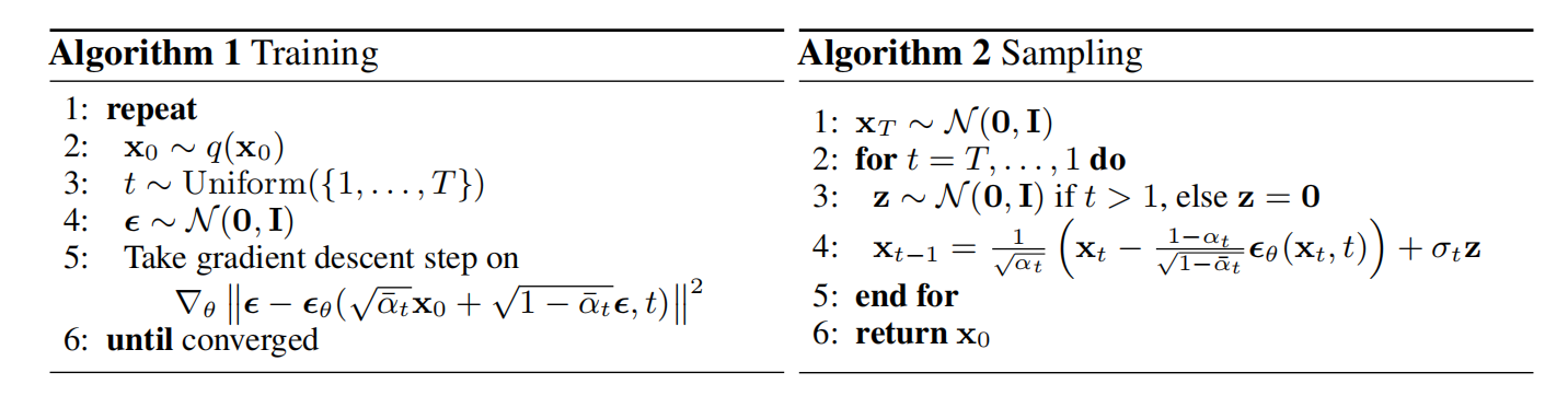
根据图2，可知，只需训练一个与时间$t$依赖的噪声近似模型$\epsilon_{\theta}$，即可得到扩散模型；采样过程与Langevin dynamics$[11]$类似，$\epsilon_{\theta}$用于学习数据密度梯度。

网络结构

DDPM模型的网络结构是在PixelCNN++基础上，利用Group Normalization替换weight normalization，整体架构类似于U-Net。

参考文献

1. Generative Modeling by Estimating Gradients of the Data Distribution | Yang Song (yang-song.net)
2. Yang L, Zhang Z, Song Y, et al. Diffusion models: A comprehensive survey of methods and applications$[J]$. ACM Computing Surveys, 2023, 56(4): 1-39.
3. Ho J, Jain A, Abbeel P. Denoising diffusion probabilistic models$[J]$. Advances in neural information processing systems, 2020, 33: 6840-6851.
4. Sohl-Dickstein J, Weiss E, Maheswaranathan N, et al. Deep unsupervised learning using nonequilibrium thermodynamics$[C]$//International conference on machine learning. PMLR, 2015: 2256-2265.
5. Song Y, Ermon S. Generative modeling by estimating gradients of the data distribution$[J]$. Advances in neural information processing systems, 2019, 32.
6. Song Y, Ermon S. Improved techniques for training score-based generative models$[J]$. Advances in neural information processing systems, 2020, 33: 12438-12448.
7. Song Y, Sohl-Dickstein J, Kingma D P, et al. Score-based generative modeling through stochastic differential equations$[J]$. arXiv preprint arXiv:2011.13456, 2020.
8. Song Y, Durkan C, Murray I, et al. Maximum likelihood training of score-based diffusion models$[J]$. Advances in Neural Information Processing Systems, 2021, 34: 1415-1428.
9. Karras T, Aittala M, Aila T, et al. Elucidating the design space of diffusion-based generative models$[J]$. Advances in Neural Information Processing Systems, 2022, 35: 26565-26577.
10. Rao–Blackwell theorem - Wikipedia
11. Evidence lower bound - Wikipedia
12. Itô diffusion - Wikipedia